LRPT decoding
Going from soft symbols to sensor images is a bit more involved than the demodulation process. This is mostly because of the limited bandwidth available, and the fact that communication is one-way, meaning that the receiver cannot signal that it has lost some data. To ensure that as many bits are recovered on the receiver side as possible, multiple layers of error correction are used, which have to be peeled back to reconstruct useable data.
The official LRPT standard description is the main reference that will be used. Another great document where you can find most of the parameters used by LRPT is the CCSDS telemetry channel coding specification. I'll also be referencing meteor_decode when describing implementation details, feel free to check out the source code for inspiration if you plan on writing your own decoder.
Step 0: synchronization
The first step to decoding is figuring out where each packet begins within the data stream. The synchronization marker is 0x1ACFFC1D, but that has been convolutionally coded (more about this later), so we have to look for the encoded equivalent. Moreover, QPSK has an intrinsic phase ambiguity: if we rotate the constellation by a multiple of 90°, it will look the same. The demodulator will lock on the carrier potentially 90°, 180°, or 270° out of phase, and the only way to figure out which offset applies is to look for all four possible rotations of the synchronization markers.
To find the synchronization marker, the stream is correlated with all possible rotations of the sync marker, and the offset with the best correlation indicates the start of a new CADU. The phase rotation can then be undone based on which rotation resulted in the highest correlation.
If differential coding is enabled, the samples stream has to be pre-processed before finding the synchronization word, since each I/Q pair encodes the difference with the previous bits rather than the bits themselves. To recover a samples stream with the expected format, cross-multiply each sample with the previous (I(t)*Q(t-1), Q(t)*I(t-1)) and take the square root of each component (diffcode/diffcode.c).
If interleaving is enabled, the first thing to do is to find the location of the interleaving marker, then de-interleave the obtained samples to undo the effects of the interleaver at the transmit side. Each bit has to be delayed by a different amount based on its offset from the latest synchronization marker (deinterleave/deinterleave.c). If i is the offset of a sample from the latest marker, its value is the value of the pre-interleaving bit at position i - (i mod 36)*36*2048.
Step 1: Viterbi decoding
One of the error correction schemes used by LRPT is convolutional coding, which effectively spreads the information contained in each bit across multiple bits, adding redundancy. This allows the receiver to find and correct bit flips caused by noise, so long as they are not too close together. The most commonly used decoder to retrieve the original bitstream is the Viterbi decoder.
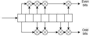
Convolutional coding works by shifting bits into a serial-to-parallel register, and XOR'ing specific outputs of the register to obtain output bits. The outputs that are combined to generate a bit are usually indicated with a connection polynomial, where each 1 bit means that the corresponding output is considered. For example, here's what the convolutional coder specified by the LRPT standard looks like:
A Viterbi decoder looks at a sequence of received symbols, and estimates the sequence of bits that most likely generated it. For each received IQ pair, it looks at all the possible states the coder might have been in, and checks the output it would have generated if a 1 was shifted in from the left or if a 0 was shifted in from the left. It then calculates how far the two generated symbols are from the one received, and adds the distance between the received pair and the generated pair to the end state's score. After some iterations of this algorithm, the state with the lowest score is picked as the most likely, and the estimated input sequence is used as the output of the decoder (ecc/viterbi.c).
For example, let's say the received symbol is (80, 100). Consider the state 0b0100010. If we assume a 1 was input, the next state would be 0b1010001, resulting in an output of 0b11 encoded as (-128, -128), while assuming the input was 0 results in the next state 0b0010001 for an output of 0b00, encoded as (127, 127). If we use the Manhattan distance as our distance metric, assuming a 1 bit results in a distance of 436, and assuming a 0 bit results in a distance of 74. We would add these numbers to the distances associated with states 0b1010001 and 0b0010001 respectively. This operation is repeated for all possible starting states, and, over time, the most likely input sequences will result in lower total state distances.
If you want to learn more about convolutional encoding and decoding, Lukas Teske has written an entry on his blog describing what he did to decode LRIT data from GOES. There are of course differences compared to LRPT, but the principle of convolutional coding is the same.
Step 2: Reed-Solomon error correction
The CADU is transmitted with added pseudorandom noise to improve the signal's spectral properties, so it has to be XOR'd again with the noise to descramble it. This noise comes from a simple linear feedback shift register (LFSR), and the generator polynomial is given, so it can be reconstructed at the receive end.
Once that is done, the second layer of error correction can be accessed. This is a Reed-Solomon code, useful to correct bursts of errors typical of the output of a convolutional decoder. As per the specification, the CADU's data section is error-corrected using 4 interleaved (255,223) Reed-Solomon codes (Reed-Solomon code n can be accessed by looking at the nth byte and every 4th byte after that, until the end of the CADU, see ecc/rs.c:58). The rest of the parameters used when encoding can be found in the CCSDS specification.
Reed-Solomon can detect and correct errors by considering the data to be coded as a sequence of coefficients of a polynomial. It then divides this polynomial by another known polynomial with some special properties, called the generator, and appends the remainder of this division to the data. At the receive side, one can check whether the data is intact by verifying that the remainder of the division matches the one received. If any byte in the message was changed (up to a certain amount), the remainder will be different, and the difference can be used to find both the position of the bytes that were corrupted as well as their original value.
If you want to learn more about the details of how to derive the error locations and magnitudes from the remainder, the Wikipedia page for Reed-Solomon error correction is a good starting point. For an example of an actual implementation, see ecc/rs.c:91
Step 3: packet field parsing
Once error-corrected, the data inside each VCDU can be parsed. Instrument data has a variable length packet unit, called MPDU, while packets at the physical layer have a fixed size. This can cause MPDUs to span more than one physical packet, so defragmentation has to be performed to get back the instrument bitstream. As seen in the MetOp documentation, each VCDU may or may not have a "MPDU first header pointer" set. If non-zero, this indicates the position of the first MPDU header in the packet. This header contains info about the size of the MPDU, which can be used to find subsequent MPDUs in the same VCDU. Note that both the header and the data of the last packet may be incomplete, with the rest of it being in the next VCDU, so take that into account when designing a defragmentation algorithm.
Step 4: JPEG decompression
MPDUs from the onboard imager (APIDs 64-69) contain 14 8x8 thumbnails (also called MCUs) each. These thumbnails are compressed using the JPEG algorithm, the parameters of which are found in the chunk's header, and are constant for all thumbnails in the chunk. Decompressing them and joining them one after the other results in the reconstruction of the scanlines from the imager.
The compression scheme is quite clearly explained in the Wikipedia page for JPEG: the Discrete Cosine Transform is computed on each 8x8 block, and the resulting coefficients are quantized and then compressed using entropy coding. The reverse process has to be applied to obtain the original image back: decompress using the JPEG Huffman tables (found here, disregard the chrominance tables and only look at luminance, annex K), rearrange the coefficients back into an 8x8 matrix, dequantize them based on the quality factor found in the header, and finally apply the Inverse Discrete Cosine Transform.
Meteor-M series deviations from the LRPT standard
For the most part, Meteor-M satellites follow the LRPT standard. Here is a list of the things I could find that are different from it:
Interleaving: the standard requires CADU bits to be interleaved using a bank of registers, and a synchronization marker added every 72 bits. This is optional for Meteor-M series satellites, and is disabled on Meteor-M2.
Differential encoding: on Meteor-M N2-2, CADU bits were differentially encoded (NRZ-M), something that is not part of the original standard. This is not the case for Meteor-M2, and may or may not be enabled for future satellites.
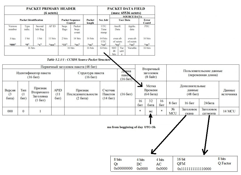
Application layer image data: compared to the format indicated for AVHRR packets, the format used by Meteor-M for MSU-MR packets is simpler to parse. Each MPDU also has a 6 byte secondary header after the primary header, followed by 14 MCUs. The MCU chunk header looks like this for image data:
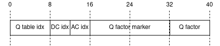
The first 16 bits are always 0, bits 16-32 are always
0xFFF0, bits 32-40 indicate the quality factor used during compression. Here is an overview image, from the now-defunct meteor.robonuka.ru. Part of it is in Russian, but you can cross-reference the images from the MetOp standard documentation to figure out what each field does. Note how each MPDU contains exactly one MCU header and exactly 14 MCUs, while the original standard allowed for more flexibility: